Comfort overlays

Comfort overlay layers evaluate thermal comfort models on the current psychrometric panel. They inherit the chart units, pressure, limits, and Mollier orientation from ggpsychro(), so comfort regions can be composed with the same + workflow as other ggplot layers.

The comfort API has three layers:

Task	API
Calculate comfort values for vectors or data frames	comfort_pmv(), comfort_set(), comfort_adaptive(), comfort_heat_index()
Store fixed model assumptions for plotting	comfort_model_pmv(), comfort_model_set(), comfort_model_adaptive(), comfort_model_heat_index()
Draw comfort fields, zones, or point metrics on a chart	geom_comfort_pmv(), geom_comfort_set(), geom_comfort_adaptive(), geom_comfort_heat_index(), geom_comfort_givoni(), stat_comfort_state()

Use the layer that matches the question you want the chart to answer:

Question	Layer
How does PMV vary across the chart?	geom_comfort_pmv()
Where are PMV-based ASHRAE 55 or EN 15251 comfort zones?	geom_comfort_pmv(standard = ...)
How does SET vary across the chart?	geom_comfort_set()
What adaptive comfort range applies for a running outdoor temperature?	geom_comfort_adaptive()
Which Outdoor Work Heat Index category applies?	geom_comfort_heat_index()
Which Givoni-Milne strategy regions apply?	geom_comfort_givoni()
What comfort metric applies to measured state points?	stat_comfort_state()

PMV overlays

The default comfort model is ISO 7730 PMV. geom_comfort_pmv() draws filled PMV bands, labelled PMV contours, and optional PMV-based standard zones. scale_fill_comfort_pmv() applies a PMV-centered diverging palette.

ggpsychro(tdb_lim = c(5, 40), hum_lim = c(0, 24)) +
    psychro_preset("minimal") +
    geom_comfort_pmv(
        contour_levels = seq(-3, 3, by = 0.5),
        n = c(70, 48)
    ) +
    scale_fill_comfort_pmv(name = "PMV")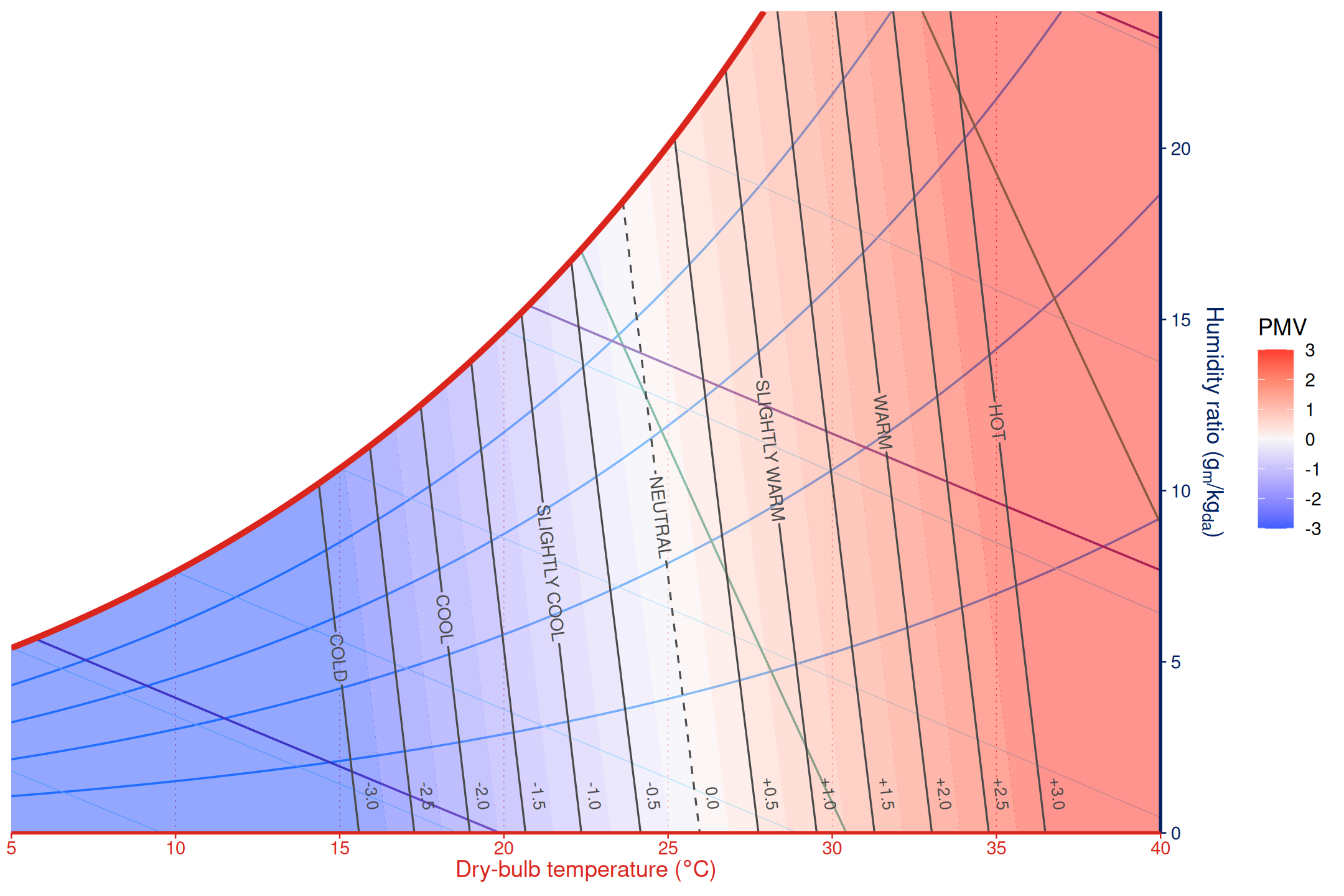

Resolution and rendering modes

Comfort layers use n as the rendering-resolution control. For filled bands, pass one value for both dry-bulb and humidity-ratio directions or two values as c(tdb, humratio). PMV contour curves use the first value because they trace constant-PMV roots along one sampling direction. Lower values build faster and are useful during exploration; higher values give smoother final graphics.

Use band_render = "band" for filled regions and band_render = "tile" for direct sampled cells. For PMV bands, band_method = "auto" uses root-traced boundaries; band_method = "isoband" uses the cheaper gridded approximation.

Default resolutions are chosen per model so the common examples build quickly while keeping smooth visible boundaries:

Layer/model	Default n	Notes
geom_comfort_pmv() bands	c(360, 220)	PMV contours and standard boundaries use the first value.
geom_comfort_set()	c(80, 50)	SET bands and contours use a sampled grid.
geom_comfort_adaptive()	c(240, 160)	Adaptive zones are sampled and clipped to the chart.
geom_comfort_heat_index()	c(160, 100)	Heat-index categories share a cached sampled grid.

Standard comfort zones

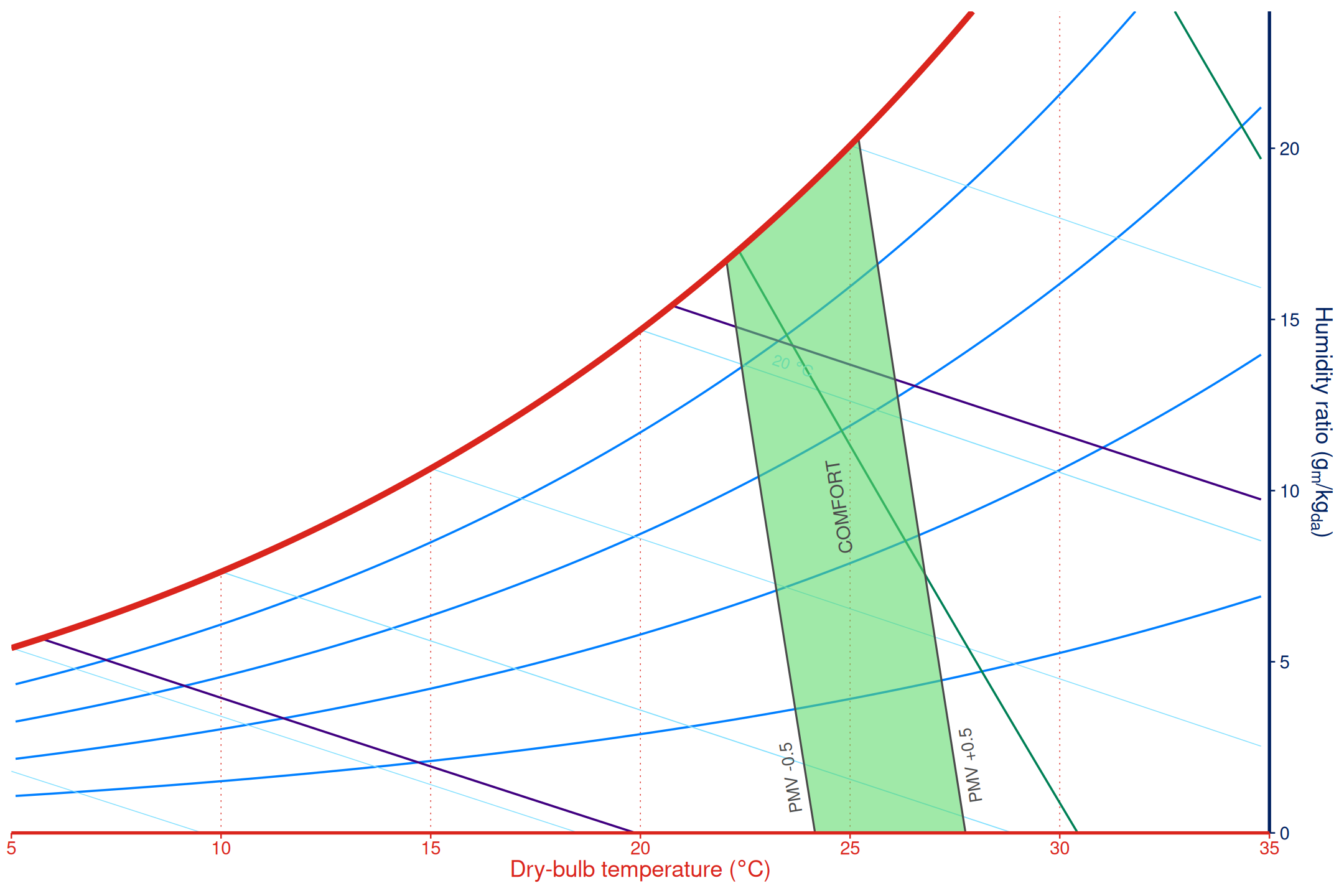
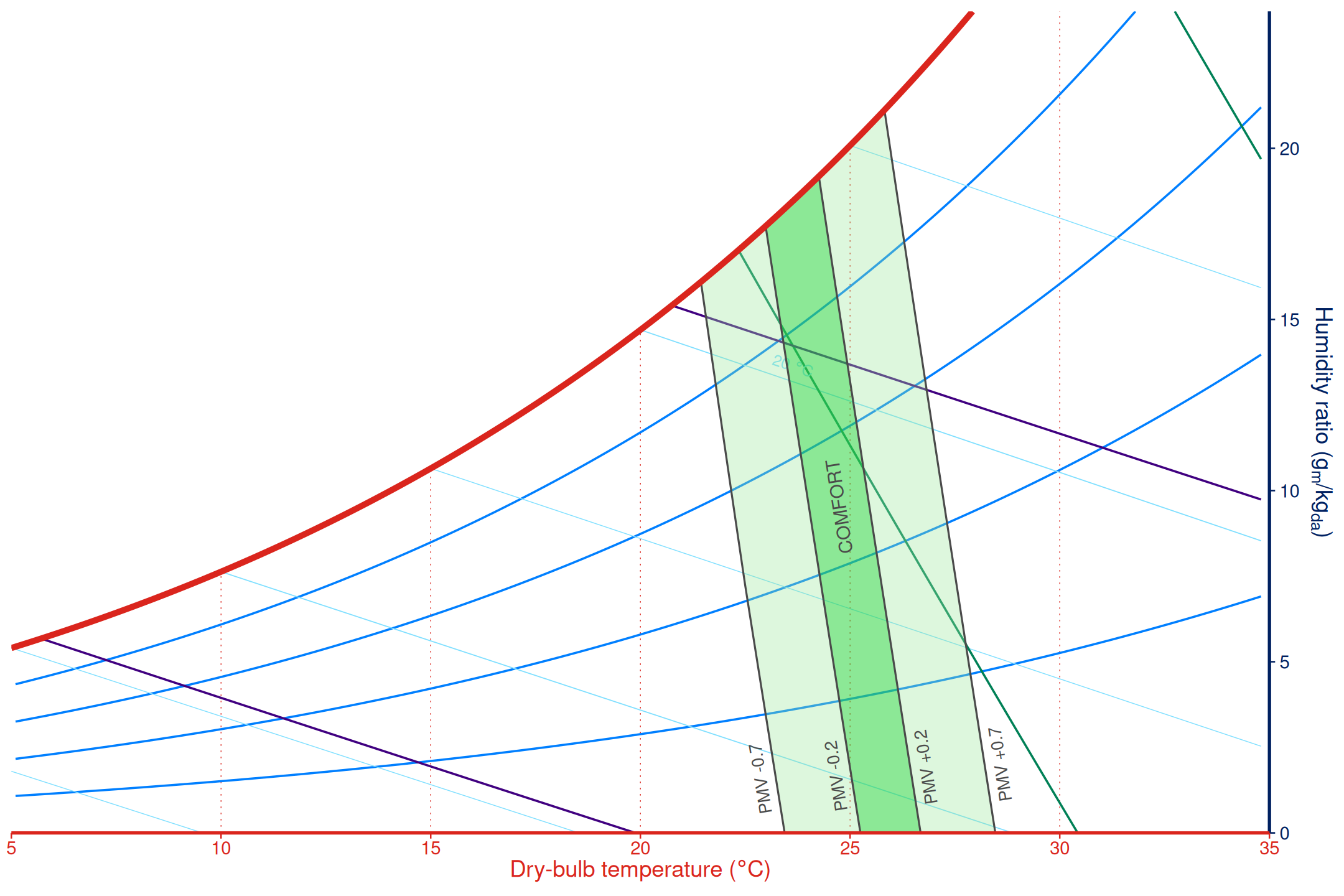
For PMV-based standards, pass a standard helper to geom_comfort_pmv(). The standard layer draws the filled zone, PMV boundary contours, and labels.

ggpsychro(tdb_lim = c(5, 35), hum_lim = c(0, 24)) +
    psychro_preset("minimal") +
    geom_comfort_pmv(
        standard = comfort_pmv_ashrae55(),
        bands = FALSE,
        contours = FALSE,
        n = 140
    )

ggpsychro(tdb_lim = c(5, 35), hum_lim = c(0, 24)) +
    psychro_preset("minimal") +
    geom_comfort_pmv(
        standard = comfort_pmv_en15251(),
        bands = FALSE,
        contours = FALSE,
        n = 140
    )

SET and adaptive models

Create reusable model objects with comfort_model_*() helpers. SET overlays default to the "set" metric, while adaptive models default to "acceptability". For continuous metrics such as SET, use filled bands with labelled contours so the field remains visible without losing the level boundaries. geom_comfort_set(contours = TRUE, labels = TRUE) draws contour labels inline and leaves a gap in each labelled contour where the label is placed.

set_model <- comfort_model_set()

ggpsychro(tdb_lim = c(15, 30), hum_lim = c(0, 20)) +
    psychro_preset("minimal") +
    geom_comfort_set(
        model = set_model,
        band_levels = seq(14, 32, by = 2),
        contours = TRUE,
        contour_levels = seq(22, 30, by = 2),
        labels = TRUE,
        n = c(70, 42),
        alpha = 0.32
    ) +
    scale_fill_viridis_c("SET (deg C)", option = "C")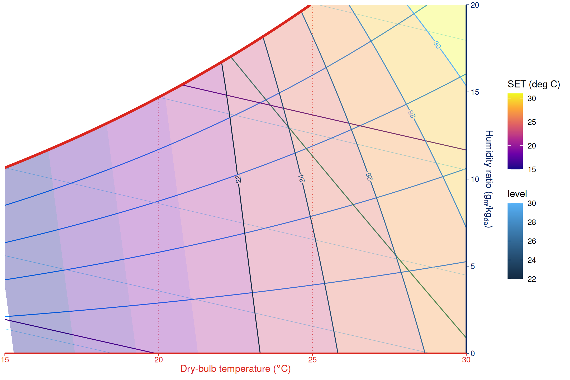

ggpsychro(tdb_lim = c(15, 30), hum_lim = c(0, 20)) +
    psychro_preset("minimal") +
    geom_comfort_adaptive(
        t_running = 20,
        fill = "#22c55e",
        alpha = 0.18,
        colour = "#166534",
        linewidth = 0.7
    )

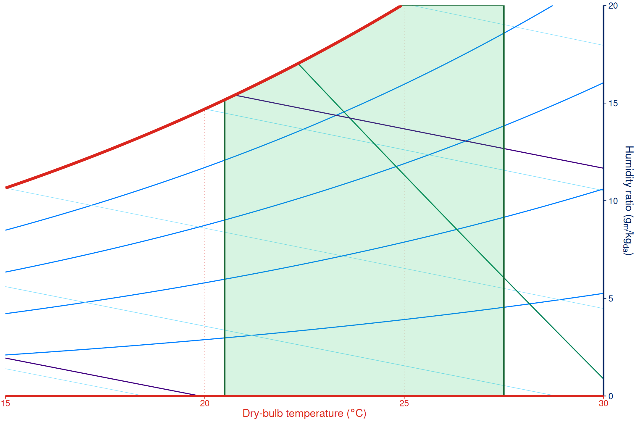
Adaptive comfort zones are temperature bands rather than humidity-dependent fields, so a filled adaptive zone is expected to look like a vertical band instead of a curved humidity field. In the example above, t_running = 20 gives an ASHRAE 55 80% acceptability interval from 20.5 to 27.5 degrees C; because tr defaults to tdb, the zone is clipped only by the current chart limits and saturation boundary.

Outdoor Heat Index

Heat Index overlays use comfort_model_heat_index() and geom_comfort_heat_index() to draw Outdoor Work Heat Index categories. The model uses a NOAA-style Heat Index calculation internally in Fahrenheit, while the layer follows the parent chart’s unit system.

ggpsychro(tdb_lim = c(20, 45), hum_lim = c(0, 35)) +
    psychro_preset("minimal") +
    geom_comfort_heat_index(n = c(70, 42), alpha = 0.5)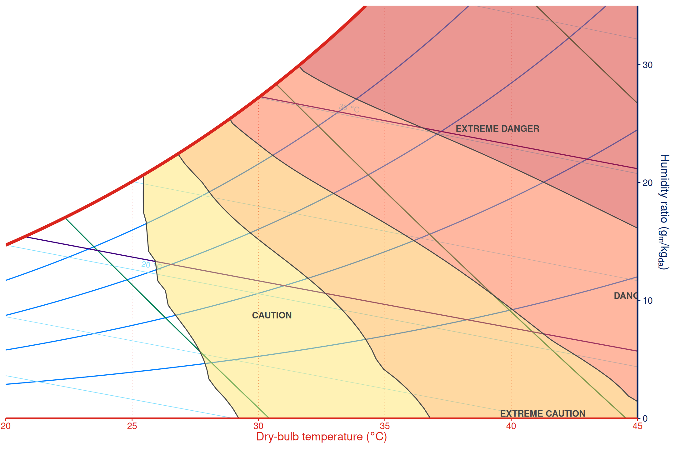

Givoni-Milne strategy overlay

Givoni-Milne overlays are strategy zones rather than a single continuous comfort metric. Create a strategy with comfort_strategy_givoni() and draw it with geom_comfort_givoni(). The default fixed variant uses the commonly cited 1979 comfort anchor of 20 to 25.5 degrees C and 20% to 80% relative humidity, with the hot-humid corner clipped. For project- or climate-specific assumptions, set tdb_range and relhum_range on the fixed variant to use those ranges as the drawing anchor. Use variant = "adaptive" and supply mean_outdoor to shift the comfort anchor from mean outdoor temperature; the adaptive layer shows that temperature as a dashed marker. Treat these regions as a pre-design screening aid: high-mass and night ventilation regions need daily profiles, nighttime conditions, and building assumptions before they can be used to count comfort hours.

givoni <- comfort_strategy_givoni()

ggpsychro(tdb_lim = c(-10, 50), hum_lim = c(0, 35)) +
    psychro_preset("minimal") +
    geom_comfort_givoni(givoni, alpha = 0.45)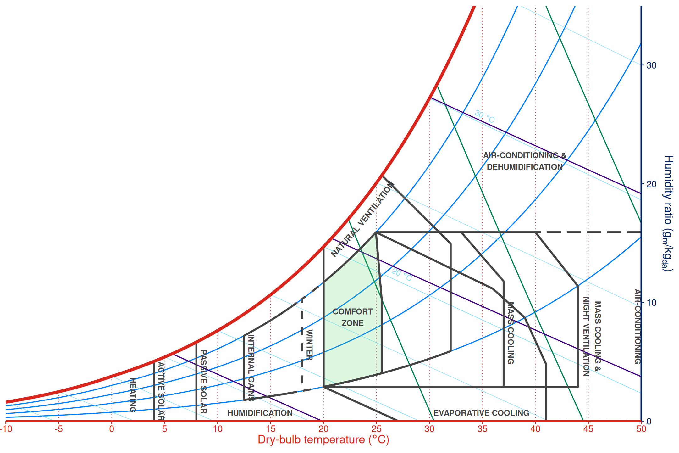

adaptive_givoni <- comfort_strategy_givoni(
    variant = "adaptive",
    mean_outdoor = 22
)

ggpsychro(tdb_lim = c(-10, 50), hum_lim = c(0, 35)) +
    psychro_preset("minimal") +
    geom_comfort_givoni(adaptive_givoni, alpha = 0.45)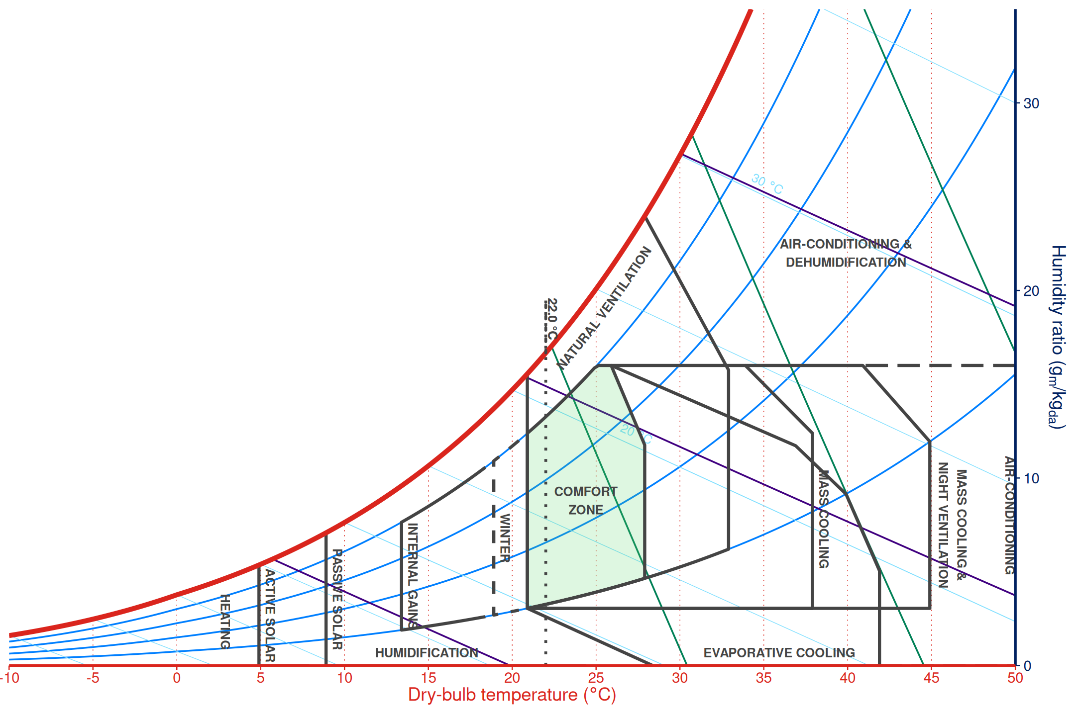

custom_givoni <- comfort_strategy_givoni(
    tdb_range = c(22, 27),
    relhum_range = c(30, 70)
)

ggpsychro(tdb_lim = c(0, 50), hum_lim = c(0, 35)) +
    psychro_preset("minimal") +
    geom_comfort_givoni(custom_givoni, alpha = 0.45)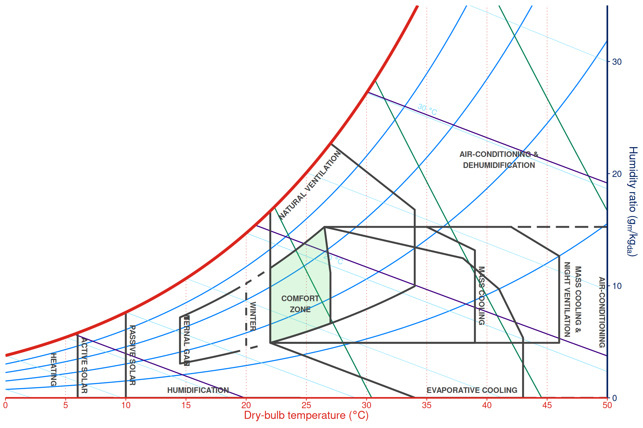

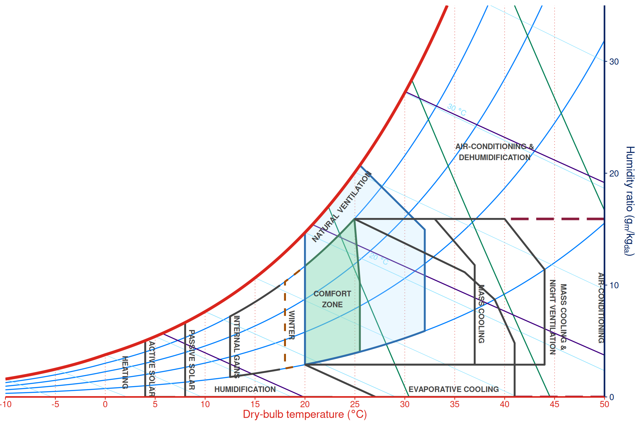
Use zone_style with element_givoni_zone() to highlight individual strategy zones without changing the strategy geometry.

ggpsychro(tdb_lim = c(-10, 50), hum_lim = c(0, 35)) +
    psychro_preset("minimal") +
    geom_comfort_givoni(
        givoni,
        zone_style = list(
            comfort = element_givoni_zone(
                fill = "#66D27A", colour = "#1F5F2D", alpha = 0.35
            ),
            natural_ventilation = element_givoni_zone(
                fill = "#B6E3FF", colour = "#2F6FB0", alpha = 0.25
            ),
            winter = element_givoni_zone(
                colour = "#A14D00", linetype = "dashed"
            ),
            air_conditioning = element_givoni_zone(
                colour = "#8B1E3F", linewidth = 1.2
            )
        )
    )

State metrics

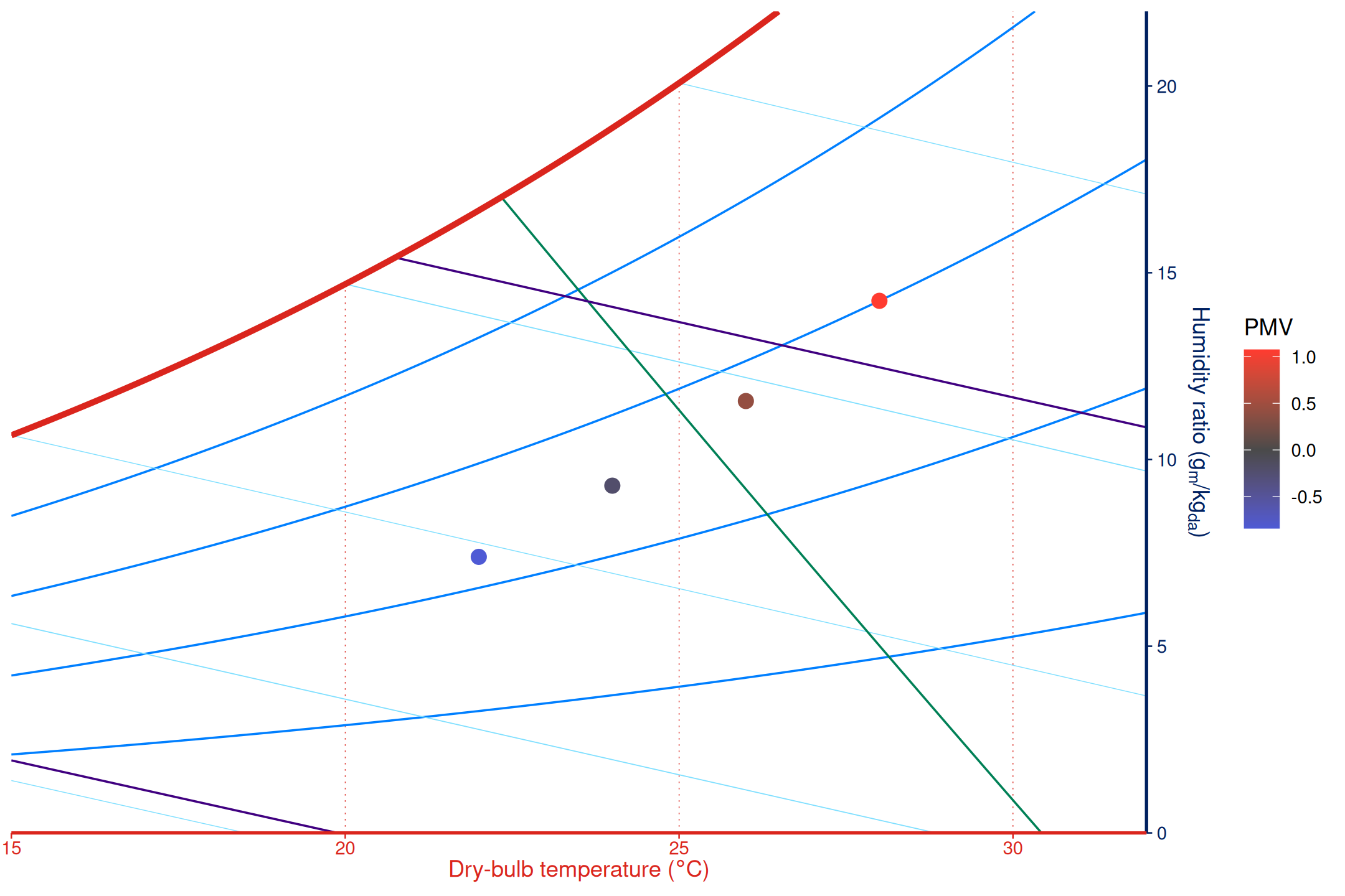
stat_comfort_state() evaluates the model at supplied psychrometric states. The computed comfort fields can be used with after_stat().

states <- data.frame(
    tdb = c(22, 24, 26, 28),
    relhum = c(45, 50, 55, 60)
)

ggpsychro(states, tdb_lim = c(15, 32), hum_lim = c(0, 22)) +
    psychro_preset("minimal") +
    stat_comfort_state(
        aes(tdb = tdb, relhum = relhum, colour = after_stat(pmv)),
        size = 3
    ) +
    scale_colour_gradient2(
        "PMV",
        low = "#3B5FFF",
        mid = "#4A4A4A",
        high = "#FF3B30",
        midpoint = 0
    )

Mollier and IP charts

Comfort layers follow the parent chart’s coordinate system. Use mollier = TRUE for Mollier orientation or units = "IP" for IP inputs.

ggpsychro(tdb_lim = c(15, 30), hum_lim = c(0, 20), mollier = TRUE) +
    psychro_preset("minimal") +
    geom_comfort_pmv(
        contour_levels = seq(-2, 2, by = 1),
        n = c(50, 30)
    ) +
    scale_fill_comfort_pmv(name = "PMV")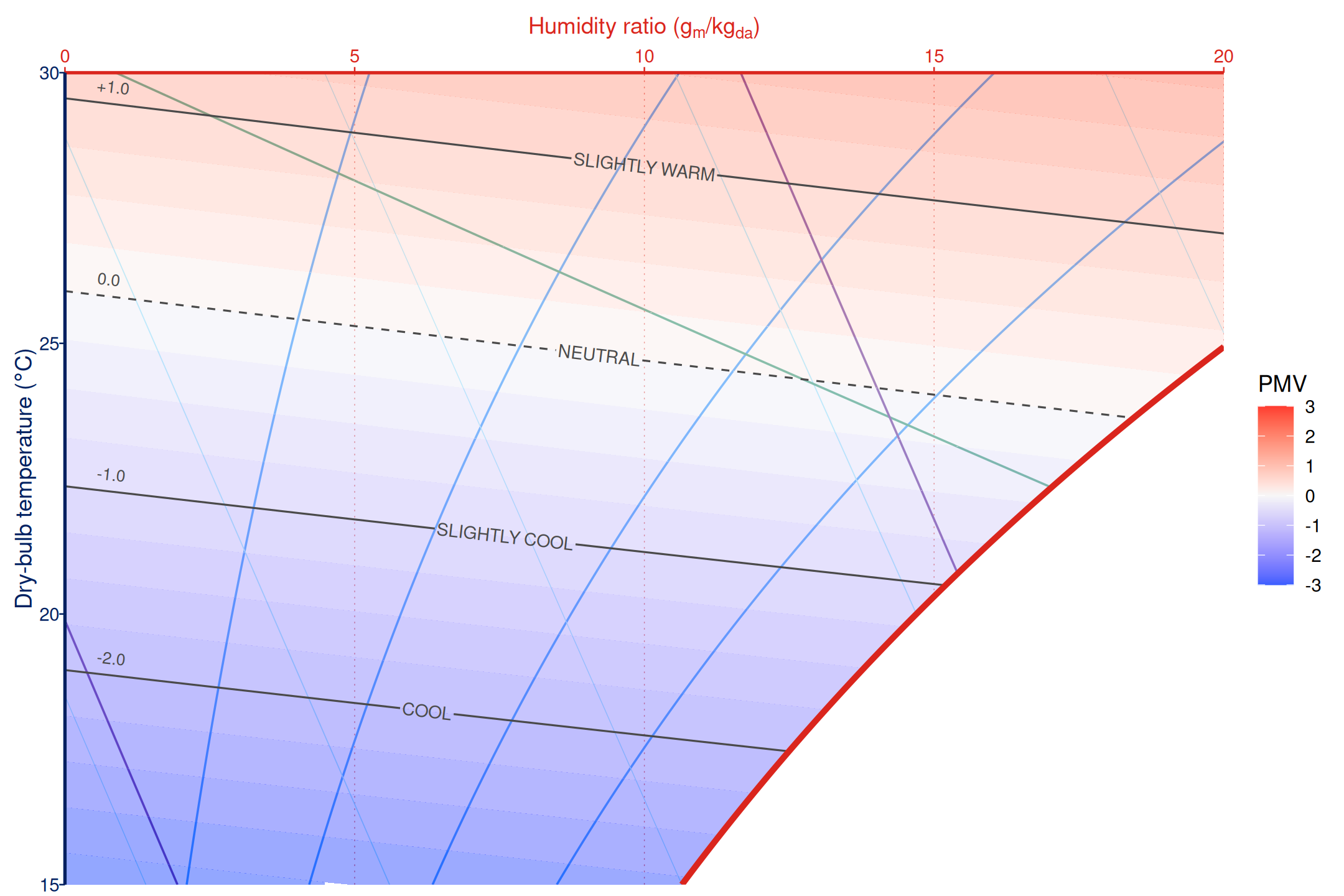

Use manual psychrometric zones when the desired region is a project-specific operating envelope rather than a thermal comfort model. See Zones and processes for those layers.