This vignette showcases the basic features of the
EplusJob class with the main focus on how the tidy data
interface can provide a seamless workflow to extract EnergyPlus output,
feed it into data analysis pipelines and turn the results into
understanding and knowledge.
Run simulations
The Idf class provides a $run() method to
call EnergyPlus and run simulations.
Idf$run() will run the current model with specified
weather using corresponding version of EnergyPlus. The model and the
weather used will be copied to the output directory. An
EplusJob object will be returned which provides detailed
information of the simulation and methods to collect simulation output.
Please see ?EplusJob for details.
eplus_ver <- max(avail_eplus())
eplus_ver
#> [1] '26.1.0'

path_idf <- file.path(eplus_config(eplus_ver)$dir, "ExampleFiles/5Zone_Transformer.idf")
path_epw <- file.path(eplus_config(eplus_ver)$dir, "WeatherData/USA_CA_San.Francisco.Intl.AP.724940_TMY3.epw")

model <- read_idf(path_idf)
#> IDD v26.1.0 has not been parsed before. Try to locate 'Energy+.idd' in
#> EnergyPlus v26.1.0 installation folder '/usr/local/EnergyPlus-26-1-0'.
#> IDD file found: '/home/runner/.local/EnergyPlus-26-1-0/Energy+.idd'.
#> Start parsing...
#> Parsing completed.
Run only design day simulation
Sometime, you may only want to run a design day simulation.
Idf$run() provides a convenient way to do this by setting
the weather argument to NULL.
job <- model$run(NULL, dir = tempdir(), wait = TRUE)
#> Adding an object in class 'Output:SQLite' and setting its 'Option Type' to
#> 'SimpleAndTabular' in order to create SQLite output file.
#> ExpandObjects Started.
#> No expanded file generated.
#> ExpandObjects Finished. Time:     0.017
#> EnergyPlus Starting
#> EnergyPlus, Version 26.1.0-6f2e40d102, YMD=2026.07.12 15:24
#> Initializing Response Factors
#> Calculating CTFs for "ROOF-1"
#> Calculating CTFs for "WALL-1"
#> Calculating CTFs for "FLOOR-SLAB-1"
#> Calculating CTFs for "INT-WALL-1"
....

class(job)
#> [1] "EplusJob" "R6"

job
#> ── EnergPlus Simulation Job ────────────────────────────────────────────────────
#>  • Path: '/home/runner/.local/EnergyPlus-26-1-0/ExampleFiles/5Zone_Transformer.…
#>  • Version: '<< Not specified >>'
#>  • EnergyPlus Version: '26.1.0'
#>  • EnergyPlus Path: '/home/runner/.local/EnergyPlus-26-1-0'
#>  Simulation started at '2026-07-12 15:24:14.738135' and completed successfully after 0.67 secs.
job prints the path of model and weather, the version
and path of EnergyPlus used to run simulations, and the simulation job
status.
You can always retrieve the last simulation job of an
Idf object using Idf$last_job() method:
model$last_job()
#> ── EnergPlus Simulation Job ────────────────────────────────────────────────────
#>  • Path: '/home/runner/.local/EnergyPlus-26-1-0/ExampleFiles/5Zone_Transformer.…
#>  • Version: '<< Not specified >>'
#>  • EnergyPlus Version: '26.1.0'
#>  • EnergyPlus Path: '/home/runner/.local/EnergyPlus-26-1-0'
#>  Simulation started at '2026-07-12 15:24:14.738135' and completed successfully after 0.67 secs.
Run simulation in the background
By default, when calling Idf$run() method, R will hang
on and wait for the simulation to complete. EnergyPlus standard output
(stdout) and error (stderr) is printed to R console. You can make
EnergyPlus run in the background by setting wait to
FALSE. The simulation job status can be shown by printing
the EplusJob object or using the
EplusJob$status() method.
job <- model$run(path_epw, tempdir(), wait = FALSE)
job
#> ── EnergPlus Simulation Job ────────────────────────────────────────────────────
#>  • Path: '/home/runner/.local/EnergyPlus-26-1-0/ExampleFiles/5Zone_Transformer.…
#>  • Version: '/home/runner/.local/EnergyPlus-26-1-0/WeatherData/USA_CA_San.Franc…
#>  • EnergyPlus Version: '26.1.0'
#>  • EnergyPlus Path: '/home/runner/.local/EnergyPlus-26-1-0'
#>  Simulation started at '2026-07-12 15:24:15.635061' and is still running...

job$status()
#> $run_before
#> [1] TRUE
#>
#> $alive
#> [1] TRUE
#>
#> $terminated
#> [1] FALSE
#>
#> $successful
#> [1] NA
#>
#> $changed_after
#> [1] FALSE
Print simulation errors
You can get simulation errors using
EplusJob$errors().
print(job$errors())
#>    index envir_index                    envir level_index   level
#>    <int>       <int>                   <char>       <int>  <char>
#> 1:     1           1 Zone Sizing Calculations           1 Warning
#> 2:     1           1 Zone Sizing Calculations           1 Warning
#> 3:     1           1 Zone Sizing Calculations           1 Warning
#> 4:     1           1 Zone Sizing Calculations           1 Warning
#> 5:     1           1 Zone Sizing Calculations           1 Warning
#>                                                                                                     message
#>                                                                                                      <char>
#> 1:                            Weather file location will be used rather than entered (IDF) Location object.
#> 2:                                                              ..Location object=CHICAGO_IL_USA TMY2-94846
#> 3:                                    ..Weather File Location=San Francisco Intl Ap CA USA TMY3 WMO#=724940
#> 4: ..due to location differences, Latitude difference=[4.16] degrees, Longitude difference=[34.65] degrees.
#> 5:             ..Time Zone difference=[2.0] hour(s), Elevation difference=[98.95] percent, [188.00] meters.
Retrieve simulation output
eplusr uses the EnergyPlus SQL output for extracting simulation
output. In order to do so, an object in Output:SQLite class
with Option Type value of SimpleAndTabular
will be automatically created if it does not exists.
EplusJob has provided some wrappers that do SQL queries to
get report data results, i.e. results from Output:Variable
and Output:Meter*. But for Output:Table
results, you have to be familiar with the structure of the EnergyPlus
SQL output, especially for table “TabularDataWithStrings”. For
details, please see “2.20 eplusout.sql”, especially
“2.20.4.4 TabularData Table” in EnergyPlus “Output Details
and Examples” documentation.
Tidy data interface
EplusJob class is designed to extract and represent
EnergyPlus simulation results from the SQLite output into tidy tables.
The layout ensures that values of different variables from the same
observation are always paired and is well fitted for data analyses using
the tidyverse R package ecosystem.
Table (a) in figure below shows an example of the standard format from EnergyPlus CSV table output, while Table (b) gives the tidy representation of the same underlying data.
Although the structure of Table (a) provides efficient storage for
completely crossed designs, it violates with the tidy principles, as
variables form both the rows and columns and column headers are values,
not variable names. Additional data cleaning efforts are needed to work
with this structure, especially considering the missing values
(NA in row 2 and 4 in Table (a)) introduced by the
aggregation of various reporting frequencies, which may add new
inefficiencies and potential errors.
In Table (b), values in column headers have been extracted and
converted into separate columns, and a new variable called
Value is used to store the concatenated data values from
the previously separate columns. Moreover, instead of presenting date
and time as strings in Table (a), the tidy data interface splits its
components into four new variables, including Month,
Day, Hour and Minute. Taken
together, Table (b) forms a nine-variable tidy table and each variable
matches the semantics of simulation output.

An example of tidy BES output data representation where Table (a) is the standard output format of EnergyPlus CSV table and Table (b) is the tidy representation of the same underlying data
Get all possible output meta data
EplusJob$report_data_dict() returns a data.table which
contains meta data of report data for current simulation. For details on
the meaning of each columns, please see “2.20.2.1
ReportDataDictionary Table” in EnergyPlus “Output Details and
Examples” documentation. The most useful columns are:
-
key_value: Key name of the data -
name: Actual report data name -
is_meter: Whether report data is a meter data. Possible values:0and1 -
reporting_frequency: Data reporting frequency -
units: The data units
print(job$report_data_dict())
#>     report_data_dictionary_index is_meter   type
#>                            <num>    <num> <char>
#>  1:                            7        0    Avg
#>  2:                            9        1    Sum
#>  3:                           21        1    Sum
#>  4:                           57        1    Sum
#>  5:                          463        1    Sum
#>  6:                          894        0    Avg
#>  7:                          895        0    Avg
#>  8:                          896        0    Sum
#>  9:                          897        0    Avg
#> 10:                          898        0    Sum
#> 11:                          899        0    Avg
#> 12:                          900        0    Sum
#> 13:                          901        0    Avg
#> 14:                          902        0    Sum
#> 15:                          903        0    Avg
#> 16:                          904        0    Sum
#> 17:                          905        0    Sum
#> 18:                          906        1    Sum
#> 19:                         1216        1    Sum
#> 20:                         1315        1    Sum
#>     report_data_dictionary_index is_meter   type
#>                            <num>    <num> <char>
#>                             index_group timestep_type     key_value
#>                                  <char>        <char>        <char>
#>  1:                                Zone          Zone   Environment
#>  2:                Facility:Electricity          Zone          <NA>
#>  3:                Building:Electricity          Zone          <NA>
#>  4: Facility:Electricity:InteriorLights          Zone          <NA>
#>  5:             Building:EnergyTransfer          Zone          <NA>
#>  6:                              System   HVAC System TRANSFORMER 1
#>  7:                              System   HVAC System TRANSFORMER 1
#>  8:                              System   HVAC System TRANSFORMER 1
#>  9:                              System   HVAC System TRANSFORMER 1
#> 10:                              System   HVAC System TRANSFORMER 1
#> 11:                              System   HVAC System TRANSFORMER 1
#> 12:                              System   HVAC System TRANSFORMER 1
#> 13:                              System   HVAC System TRANSFORMER 1
#> 14:                              System   HVAC System TRANSFORMER 1
#> 15:                              System   HVAC System TRANSFORMER 1
#> 16:                              System   HVAC System TRANSFORMER 1
#> 17:                              System   HVAC System TRANSFORMER 1
#> 18:                    HVAC:Electricity          Zone          <NA>
#> 19:           Facility:Electricity:Fans          Zone          <NA>
#> 20:                   Plant:Electricity          Zone          <NA>
#>                             index_group timestep_type     key_value
#>                                  <char>        <char>        <char>
#>                                                 name reporting_frequency
#>                                               <char>              <char>
#>  1:             Site Outdoor Air Drybulb Temperature       Zone Timestep
#>  2:                             Electricity:Facility       Zone Timestep
#>  3:                             Electricity:Building       Zone Timestep
#>  4:                       InteriorLights:Electricity       Zone Timestep
#>  5:                          EnergyTransfer:Building       Zone Timestep
#>  6:                           Transformer Efficiency       Zone Timestep
#>  7:               Transformer Input Electricity Rate       Zone Timestep
#>  8:             Transformer Input Electricity Energy       Zone Timestep
#>  9:              Transformer Output Electricity Rate       Zone Timestep
#> 10:            Transformer Output Electricity Energy       Zone Timestep
#> 11:                    Transformer No Load Loss Rate       Zone Timestep
#> 12:                  Transformer No Load Loss Energy       Zone Timestep
#> 13:                       Transformer Load Loss Rate       Zone Timestep
#> 14:                     Transformer Load Loss Energy       Zone Timestep
#> 15:                    Transformer Thermal Loss Rate       Zone Timestep
#> 16:                  Transformer Thermal Loss Energy       Zone Timestep
#> 17: Transformer Distribution Electricity Loss Energy       Zone Timestep
#> 18:                                 Electricity:HVAC       Zone Timestep
#> 19:                                 Fans:Electricity       Zone Timestep
#> 20:                                Electricity:Plant       Zone Timestep
#>                                                 name reporting_frequency
#>                                               <char>              <char>
#>     schedule_name  units
#>            <char> <char>
#>  1:          <NA>      C
#>  2:          <NA>      J
#>  3:          <NA>      J
#>  4:          <NA>      J
#>  5:          <NA>      J
#>  6:          <NA>
#>  7:          <NA>      W
#>  8:          <NA>      J
#>  9:          <NA>      W
#> 10:          <NA>      J
#> 11:          <NA>      W
#> 12:          <NA>      J
#> 13:          <NA>      W
#> 14:          <NA>      J
#> 15:          <NA>      W
#> 16:          <NA>      J
#> 17:          <NA>      J
#> 18:          <NA>      J
#> 19:          <NA>      J
#> 20:          <NA>      J
#>     schedule_name  units
#>            <char> <char>
Retrieve report data
EplusJob$report_data() extracts the report data using
key values and variable names. Just for demonstration, let’s get the
transformer input electric power at 11 a.m for the first day of
RunPeriod named SUMMERDAY, tag this simulation as case
example, and return all possible output columns.
power <- job$report_data("transformer 1", "transformer input electric power", case = "example",
  all = TRUE, simulation_days = 1, environment_name = "summerday", hour = 11, minute = 0)

print(power)
#> Empty data.table (0 rows and 22 cols): case,datetime,month,day,hour,minute...
Please note that by default the report data of design day simulations are always put at the top. If you are only interested in results of specific run periods, there are 2 ways to do so:
- Set
environment_nameto the run periods you are interested, e.g.:
job$report_data(environment_name = c("summerday", "winterday"))
#>                    case            datetime   key_value
#>                  <char>              <POSc>      <char>
#>    1: 5Zone_Transformer 2014-01-14 00:15:00 Environment
#>    2: 5Zone_Transformer 2014-01-14 00:30:00 Environment
#>    3: 5Zone_Transformer 2014-01-14 00:45:00 Environment
#>    4: 5Zone_Transformer 2014-01-14 01:00:00 Environment
#>    5: 5Zone_Transformer 2014-01-14 01:15:00 Environment
#>   ---
#> 3836: 5Zone_Transformer 2015-07-07 23:00:00        <NA>
#> 3837: 5Zone_Transformer 2015-07-07 23:15:00        <NA>
#> 3838: 5Zone_Transformer 2015-07-07 23:30:00        <NA>
#> 3839: 5Zone_Transformer 2015-07-07 23:45:00        <NA>
#> 3840: 5Zone_Transformer 2015-07-08 00:00:00        <NA>
#>                                       name  units value
#>                                     <char> <char> <num>
#>    1: Site Outdoor Air Drybulb Temperature      C 9.900
#>    2: Site Outdoor Air Drybulb Temperature      C 9.200
#>    3: Site Outdoor Air Drybulb Temperature      C 8.500
#>    4: Site Outdoor Air Drybulb Temperature      C 7.800
#>    5: Site Outdoor Air Drybulb Temperature      C 8.075
#>   ---
#> 3836:                    Electricity:Plant      J 0.000
#> 3837:                    Electricity:Plant      J 0.000
#> 3838:                    Electricity:Plant      J 0.000
#> 3839:                    Electricity:Plant      J 0.000
#> 3840: Electricity:Plant J 0.000- Set
day_typeto specific day types you are interested. A few grouped options are also provided:-
"Weekday": All working days, i.e. from"Monday"to"Friday" -
"Weekend":"Saturday"and"Sunday" -
"DesignDay": Equivalent to"SummerDesignDay"plus"WinterDesignDay" -
"CustomDay":"CustomDay1"and"CustomDay2" -
"SpecialDay": Equivalent to"DesignDay"plus"CustomDay" -
"NormalDay": Equivalent to"Weekday"and"Weekend"plus"Holiday"
-
job$report_data(day_type = "normalday")
#>                    case            datetime   key_value
#>                  <char>              <POSc>      <char>
#>    1: 5Zone_Transformer 2014-01-14 00:15:00 Environment
#>    2: 5Zone_Transformer 2014-01-14 00:30:00 Environment
#>    3: 5Zone_Transformer 2014-01-14 00:45:00 Environment
#>    4: 5Zone_Transformer 2014-01-14 01:00:00 Environment
#>    5: 5Zone_Transformer 2014-01-14 01:15:00 Environment
#>   ---
#> 3836: 5Zone_Transformer 2015-07-07 23:00:00        <NA>
#> 3837: 5Zone_Transformer 2015-07-07 23:15:00        <NA>
#> 3838: 5Zone_Transformer 2015-07-07 23:30:00        <NA>
#> 3839: 5Zone_Transformer 2015-07-07 23:45:00        <NA>
#> 3840: 5Zone_Transformer 2015-07-08 00:00:00        <NA>
#>                                       name  units value
#>                                     <char> <char> <num>
#>    1: Site Outdoor Air Drybulb Temperature      C 9.900
#>    2: Site Outdoor Air Drybulb Temperature      C 9.200
#>    3: Site Outdoor Air Drybulb Temperature      C 8.500
#>    4: Site Outdoor Air Drybulb Temperature      C 7.800
#>    5: Site Outdoor Air Drybulb Temperature      C 8.075
#>   ---
#> 3836:                    Electricity:Plant      J 0.000
#> 3837:                    Electricity:Plant      J 0.000
#> 3838:                    Electricity:Plant      J 0.000
#> 3839:                    Electricity:Plant      J 0.000
#> 3840:                    Electricity:Plant      J 0.000
$report_data() can also directly take the whole or
subset results of $report_data_dict() to extract report
data. In some case this may be quite handy. Let’s get all report
variable with Celsius degree unit.
print(job$report_data(job$report_data_dict()[units == "C"]))
#>                   case            datetime   key_value
#>                 <char>              <POSc>      <char>
#>   1: 5Zone_Transformer 2014-01-14 00:15:00 Environment
#>   2: 5Zone_Transformer 2014-01-14 00:30:00 Environment
#>   3: 5Zone_Transformer 2014-01-14 00:45:00 Environment
#>   4: 5Zone_Transformer 2014-01-14 01:00:00 Environment
#>   5: 5Zone_Transformer 2014-01-14 01:15:00 Environment
#>  ---
#> 188: 5Zone_Transformer 2015-07-07 23:00:00 Environment
#> 189: 5Zone_Transformer 2015-07-07 23:15:00 Environment
#> 190: 5Zone_Transformer 2015-07-07 23:30:00 Environment
#> 191: 5Zone_Transformer 2015-07-07 23:45:00 Environment
#> 192: 5Zone_Transformer 2015-07-08 00:00:00 Environment
#>                                      name  units  value
#>                                    <char> <char>  <num>
#>   1: Site Outdoor Air Drybulb Temperature      C  9.900
#>   2: Site Outdoor Air Drybulb Temperature      C  9.200
#>   3: Site Outdoor Air Drybulb Temperature      C  8.500
#>   4: Site Outdoor Air Drybulb Temperature      C  7.800
#>   5: Site Outdoor Air Drybulb Temperature      C  8.075
#>  ---
#> 188: Site Outdoor Air Drybulb Temperature      C 15.200
#> 189: Site Outdoor Air Drybulb Temperature      C 15.100
#> 190: Site Outdoor Air Drybulb Temperature      C 15.000
#> 191: Site Outdoor Air Drybulb Temperature      C 14.900
#> 192: Site Outdoor Air Drybulb Temperature      C 14.800
Retrieve tabular data
EplusJob$tabular_data() extracts tabular data of current
simulation. For details on the meaning of each columns, please see
“2.20.4.4 TabularData Table” in EnergyPlus “Output Details
and Examples” documentation.
Now let’s get the total site energy per total building area. Note
that the value column in the returned
data.table is character types, as some table store not just
numbers. We need to convert it by setting string_value to
FALSE.
site_energy <- job$tabular_data(
    column_name = "energy per total building area", row_name = "total site energy",
    wide = TRUE, string_value = FALSE
)[[1]]
print(site_energy)
#> Key: <case, report_name, report_for, table_name>
#>                 case                             report_name      report_for
#>               <char>                                  <char>          <char>
#> 1: 5Zone_Transformer AnnualBuildingUtilityPerformanceSummary Entire Facility
#>                table_name          row_name
#>                    <char>            <char>
#> 1: Site and Source Energy Total Site Energy
#>    Energy Per Total Building Area [MJ/m2]
#>                                     <num>
#> 1:                                   1.44
Data exploration example
Data exploration is an essential aspect of building energy simulation. In this example, we will demonstrates the data exploration process of obtaining:
- energy use intensity (EUI)
- heating and cooling demand profile
Run annual simulation
path_model <- file.path(eplus_config(eplus_ver)$dir, "ExampleFiles/RefBldgMediumOfficeNew2004_Chicago.idf")
path_weather <- file.path(eplus_config(eplus_ver)$dir, "WeatherData/USA_IL_Chicago-OHare.Intl.AP.725300_TMY3.epw")

idf <- read_idf(path_model)

# make sure weather file input is respected
idf$SimulationControl$Run_Simulation_for_Weather_File_Run_Periods <- "Yes"

# make sure energy consumption is presented in kWh
idf$OutputControl_Table_Style$Unit_Conversion <- "JtoKWH"

# save the modified model into a temporary folder
idf$save(file.path(tempdir(), "MediumOffice.idf"), overwrite = TRUE)

# run annual simulation
job <- idf$run(path_weather, echo = FALSE)
Extract simulation results
Code below shows how to use methods tabular_data(),
read_table() and report_data() provided by the
tidy data interface in EplusJob to extract building area
and building energy consumption, zone meta data, and cooling and heating
demands, with all formatted in a tidy representation.
Note that instead of presenting the simulated date and time as
strings, the report_data() adds a time-series column
datetime in POSIXct based on a derived year
value. Moreover, the tidy data interface also provides a number of
additional columns, which makes it quite convenient and straightforward
to directly perform further data transformations.
# read building area from Standard Reports
print(area <- job$tabular_data(table_name = "Building Area", wide = TRUE)[[1L]])
#> Key: <case, report_name, report_for, table_name>
#> case report_name report_for
#> <char> <char> <char>
#> 1: MediumOffice AnnualBuildingUtilityPerformanceSummary Entire Facility
#> 2: MediumOffice AnnualBuildingUtilityPerformanceSummary Entire Facility
#> 3: MediumOffice AnnualBuildingUtilityPerformanceSummary Entire Facility
#> table_name row_name Area [m2]
#> <char> <char> <num>
#> 1: Building Area Total Building Area 4982.19
#> 2: Building Area Net Conditioned Building Area 4982.19
#> 3: Building Area Unconditioned Building Area 0.00
# read building energy consumption from Standard Reports
print(end_use <- job$tabular_data(table_name = "End Uses", wide = TRUE)[[1L]])
#> Key: <case, report_name, report_for, table_name>
#> case report_name report_for
#> <char> <char> <char>
#> 1: MediumOffice AnnualBuildingUtilityPerformanceSummary Entire Facility
#> 2: MediumOffice AnnualBuildingUtilityPerformanceSummary Entire Facility
#> 3: MediumOffice AnnualBuildingUtilityPerformanceSummary Entire Facility
#> 4: MediumOffice AnnualBuildingUtilityPerformanceSummary Entire Facility
#> 5: MediumOffice AnnualBuildingUtilityPerformanceSummary Entire Facility
#> 6: MediumOffice AnnualBuildingUtilityPerformanceSummary Entire Facility
#> 7: MediumOffice AnnualBuildingUtilityPerformanceSummary Entire Facility
#> 8: MediumOffice AnnualBuildingUtilityPerformanceSummary Entire Facility
#> 9: MediumOffice AnnualBuildingUtilityPerformanceSummary Entire Facility
#> 10: MediumOffice AnnualBuildingUtilityPerformanceSummary Entire Facility
#> 11: MediumOffice AnnualBuildingUtilityPerformanceSummary Entire Facility
#> 12: MediumOffice AnnualBuildingUtilityPerformanceSummary Entire Facility
#> 13: MediumOffice AnnualBuildingUtilityPerformanceSummary Entire Facility
#> 14: MediumOffice AnnualBuildingUtilityPerformanceSummary Entire Facility
#> 15: MediumOffice AnnualBuildingUtilityPerformanceSummary Entire Facility
#> table_name row_name Electricity [kWh] Natural Gas [kWh]
#> <char> <char> <num> <num>
#> 1: End Uses Heating 142077.61 50331.57
#> 2: End Uses Cooling 76542.52 0.00
#> 3: End Uses Interior Lighting 168399.82 0.00
#> 4: End Uses Exterior Lighting 64602.19 0.00
#> 5: End Uses Interior Equipment 296261.61 0.00
#> 6: End Uses Exterior Equipment 0.00 0.00
#> 7: End Uses Fans 20001.42 0.00
#> 8: End Uses Pumps 73.94 0.00
#> 9: End Uses Heat Rejection 0.00 0.00
#> 10: End Uses Humidification 0.00 0.00
#> 11: End Uses Heat Recovery 0.00 0.00
#> 12: End Uses Water Systems 0.00 10029.69
#> 13: End Uses Refrigeration 0.00 0.00
#> 14: End Uses Generators 0.00 0.00
#> 15: End Uses Total End Uses 767959.11 60361.26
#> Gasoline [kWh] Diesel [kWh] Coal [kWh] Fuel Oil No 1 [kWh]
#> <num> <num> <num> <num>
#> 1: 0 0 0 0
#> 2: 0 0 0 0
#> 3: 0 0 0 0
#> 4: 0 0 0 0
#> 5: 0 0 0 0
#> 6: 0 0 0 0
#> 7: 0 0 0 0
#> 8: 0 0 0 0
#> 9: 0 0 0 0
#> 10: 0 0 0 0
#> 11: 0 0 0 0
#> 12: 0 0 0 0
#> 13: 0 0 0 0
#> 14: 0 0 0 0
#> 15: 0 0 0 0
#> Fuel Oil No 2 [kWh] Propane [kWh] Other Fuel 1 [kWh] Other Fuel 2 [kWh]
#> <num> <num> <num> <num>
#> 1: 0 0 0 0
#> 2: 0 0 0 0
#> 3: 0 0 0 0
#> 4: 0 0 0 0
#> 5: 0 0 0 0
#> 6: 0 0 0 0
#> 7: 0 0 0 0
#> 8: 0 0 0 0
#> 9: 0 0 0 0
#> 10: 0 0 0 0
#> 11: 0 0 0 0
#> 12: 0 0 0 0
#> 13: 0 0 0 0
#> 14: 0 0 0 0
#> 15: 0 0 0 0
#> District Cooling [kWh] District Heating Water [kWh]
#> <num> <num>
#> 1: 0 0
#> 2: 0 0
#> 3: 0 0
#> 4: 0 0
#> 5: 0 0
#> 6: 0 0
#> 7: 0 0
#> 8: 0 0
#> 9: 0 0
#> 10: 0 0
#> 11: 0 0
#> 12: 0 0
#> 13: 0 0
#> 14: 0 0
#> 15: 0 0
#> District Heating Steam [kWh] Water [m3]
#> <num> <num>
#> 1: 0 0.00
#> 2: 0 0.00
#> 3: 0 0.00
#> 4: 0 0.00
#> 5: 0 0.00
#> 6: 0 0.00
#> 7: 0 0.00
#> 8: 0 0.00
#> 9: 0 0.00
#> 10: 0 0.00
#> 11: 0 0.00
#> 12: 0 174.59
#> 13: 0 0.00
#> 14: 0 0.00
#> 15: 0 174.59
# read zone metadata from Standard Input and Output
print(zones <- job$read_table("Zones"))
#> zone_index zone_name rel_north origin_x origin_y origin_z
#> <num> <char> <num> <num> <num> <num>
#> 1: 1 CORE_BOTTOM 0 0 0 0
#> 2: 2 CORE_MID 0 0 0 0
#> 3: 3 CORE_TOP 0 0 0 0
#> 4: 4 FIRSTFLOOR_PLENUM 0 0 0 0
#> 5: 5 MIDFLOOR_PLENUM 0 0 0 0
#> 6: 6 PERIMETER_BOT_ZN_1 0 0 0 0
#> 7: 7 PERIMETER_BOT_ZN_2 0 0 0 0
#> 8: 8 PERIMETER_BOT_ZN_3 0 0 0 0
#> 9: 9 PERIMETER_BOT_ZN_4 0 0 0 0
#> 10: 10 PERIMETER_MID_ZN_1 0 0 0 0
#> 11: 11 PERIMETER_MID_ZN_2 0 0 0 0
#> 12: 12 PERIMETER_MID_ZN_3 0 0 0 0
#> 13: 13 PERIMETER_MID_ZN_4 0 0 0 0
#> 14: 14 PERIMETER_TOP_ZN_1 0 0 0 0
#> 15: 15 PERIMETER_TOP_ZN_2 0 0 0 0
#> 16: 16 PERIMETER_TOP_ZN_3 0 0 0 0
#> 17: 17 PERIMETER_TOP_ZN_4 0 0 0 0
#> 18: 18 TOPFLOOR_PLENUM 0 0 0 0
#> centroid_x centroid_y centroid_z of_type multiplier list_multiplier
#> <num> <num> <num> <num> <num> <num>
#> 1: 24.955350 16.636900 1.3716 1 1 1
#> 2: 24.955350 16.636900 5.3340 1 1 1
#> 3: 24.955350 16.636900 9.2964 1 1 1
#> 4: 24.955500 16.636900 3.3528 1 1 1
#> 5: 24.955500 16.636900 7.3152 1 1 1
#> 6: 24.955448 2.158891 1.3716 1 1 1
#> 7: 47.820225 16.636900 1.3716 1 1 1
#> 8: 24.955448 31.114909 1.3716 1 1 1
#> 9: 2.090634 16.636900 1.3716 1 1 1
#> 10: 24.955448 2.158891 5.3340 1 1 1
#> 11: 47.820225 16.636900 5.3340 1 1 1
#> 12: 24.955448 31.114909 5.3340 1 1 1
#> 13: 2.090634 16.636900 5.3340 1 1 1
#> 14: 24.955448 2.158891 9.2964 1 1 1
#> 15: 47.820225 16.636900 9.2964 1 1 1
#> 16: 24.955448 31.114909 9.2964 1 1 1
#> 17: 2.090634 16.636900 9.2964 1 1 1
#> 18: 24.955500 16.636900 11.2776 1 1 1
#> minimum_x maximum_x minimum_y maximum_y minimum_z maximum_z ceiling_height
#> <num> <num> <num> <num> <num> <num> <num>
#> 1: 4.5732 45.3375 4.5732 28.7006 0.0000 2.7432 2.7432
#> 2: 4.5732 45.3375 4.5732 28.7006 3.9624 6.7056 2.7432
#> 3: 4.5732 45.3375 4.5732 28.7006 7.9248 10.6680 2.7432
#> 4: 0.0000 49.9110 0.0000 33.2738 2.7432 3.9624 1.2192
#> 5: 0.0000 49.9110 0.0000 33.2738 6.7056 7.9248 1.2192
#> 6: 0.0000 49.9110 0.0000 4.5732 0.0000 2.7432 2.7432
#> 7: 45.3375 49.9110 0.0000 33.2738 0.0000 2.7432 2.7432
#> 8: 0.0000 49.9110 28.7006 33.2738 0.0000 2.7432 2.7432
#> 9: 0.0000 4.5732 0.0000 33.2738 0.0000 2.7432 2.7432
#> 10: 0.0000 49.9110 0.0000 4.5732 3.9624 6.7056 2.7432
#> 11: 45.3375 49.9110 0.0000 33.2738 3.9624 6.7056 2.7432
#> 12: 0.0000 49.9110 28.7006 33.2738 3.9624 6.7056 2.7432
#> 13: 0.0000 4.5732 0.0000 33.2738 3.9624 6.7056 2.7432
#> 14: 0.0000 49.9110 0.0000 4.5732 7.9248 10.6680 2.7432
#> 15: 45.3375 49.9110 0.0000 33.2738 7.9248 10.6680 2.7432
#> 16: 0.0000 49.9110 28.7006 33.2738 7.9248 10.6680 2.7432
#> 17: 0.0000 4.5732 0.0000 33.2738 7.9248 10.6680 2.7432
#> 18: 0.0000 49.9110 0.0000 33.2738 10.6680 11.8872 1.2192
#> volume inside_convection_algo outside_convection_algo floor_area
#> <num> <num> <num> <num>
#> 1: 2698.0375 2 7 983.5366
#> 2: 2698.0375 2 7 983.5366
#> 3: 2698.0375 2 7 983.5366
#> 4: 2024.7603 2 7 1660.7286
#> 5: 2024.7603 2 7 1660.7286
#> 6: 568.7700 2 7 207.3381
#> 7: 360.0785 2 7 131.2622
#> 8: 568.7700 2 7 207.3381
#> 9: 360.0548 2 7 131.2536
#> 10: 568.7700 2 7 207.3381
#> 11: 360.0785 2 7 131.2622
#> 12: 568.7700 2 7 207.3381
#> 13: 360.0548 2 7 131.2536
#> 14: 568.7700 2 7 207.3381
#> 15: 360.0785 2 7 131.2622
#> 16: 568.7700 2 7 207.3381
#> 17: 360.0548 2 7 131.2536
#> 18: 2024.7603 2 7 1660.7286
#> ext_gross_wall_area ext_net_wall_area ext_window_area is_part_of_total_area
#> <num> <num> <num> <num>
#> 1: 0.00000 0.00000 0.00000 1
#> 2: 0.00000 0.00000 0.00000 1
#> 3: 0.00000 0.00000 0.00000 1
#> 4: 202.83782 202.83782 0.00000 0
#> 5: 202.83782 202.83782 0.00000 0
#> 6: 136.91586 71.63358 65.28228 1
#> 7: 91.27669 47.75469 43.52200 1
#> 8: 136.91586 71.63358 65.28228 1
#> 9: 91.27669 47.75469 43.52200 1
#> 10: 136.91586 71.63358 65.28228 1
#> 11: 91.27669 47.75469 43.52200 1
#> 12: 136.91586 71.63358 65.28228 1
#> 13: 91.27669 47.75469 43.52200 1
#> 14: 136.91586 71.63358 65.28228 1
#> 15: 91.27669 47.75469 43.52200 1
#> 16: 136.91586 71.63358 65.28228 1
#> 17: 91.27669 47.75469 43.52200 1
#> 18: 202.83782 202.83782 0.00000 0
# read hourly air-conditioning system output with all additional metadata for
# the annual simulation from Variable Output
print(aircon_out <- job$report_data(
name = sprintf("air system total %s energy", c("heating", "cooling")),
environment_name = "annual",
all = TRUE
))
#> case datetime month day hour minute dst interval
#> <char> <POSc> <num> <num> <num> <num> <num> <num>
#> 1: MediumOffice 2017-01-01 01:00:00 1 1 1 0 0 60
#> 2: MediumOffice 2017-01-01 02:00:00 1 1 2 0 0 60
#> 3: MediumOffice 2017-01-01 03:00:00 1 1 3 0 0 60
#> 4: MediumOffice 2017-01-01 04:00:00 1 1 4 0 0 60
#> 5: MediumOffice 2017-01-01 05:00:00 1 1 5 0 0 60
#> ---
#> 52556: MediumOffice 2017-12-31 20:00:00 12 31 20 0 0 60
#> 52557: MediumOffice 2017-12-31 21:00:00 12 31 21 0 0 60
#> 52558: MediumOffice 2017-12-31 22:00:00 12 31 22 0 0 60
#> 52559: MediumOffice 2017-12-31 23:00:00 12 31 23 0 0 60
#> 52560: MediumOffice 2018-01-01 00:00:00 12 31 24 0 0 60
#> simulation_days day_type environment_name environment_period_index
#> <num> <char> <char> <num>
#> 1: 1 Holiday ANNUAL 3
#> 2: 1 Holiday ANNUAL 3
#> 3: 1 Holiday ANNUAL 3
#> 4: 1 Holiday ANNUAL 3
#> 5: 1 Holiday ANNUAL 3
#> ---
#> 52556: 365 Sunday ANNUAL 3
#> 52557: 365 Sunday ANNUAL 3
#> 52558: 365 Sunday ANNUAL 3
#> 52559: 365 Sunday ANNUAL 3
#> 52560: 365 Sunday ANNUAL 3
#> is_meter type index_group timestep_type key_value
#> <num> <char> <char> <char> <char>
#> 1: 0 Sum System HVAC System VAV_1
#> 2: 0 Sum System HVAC System VAV_1
#> 3: 0 Sum System HVAC System VAV_1
#> 4: 0 Sum System HVAC System VAV_1
#> 5: 0 Sum System HVAC System VAV_1
#> ---
#> 52556: 0 Sum System HVAC System VAV_3
#> 52557: 0 Sum System HVAC System VAV_3
#> 52558: 0 Sum System HVAC System VAV_3
#> 52559: 0 Sum System HVAC System VAV_3
#> 52560: 0 Sum System HVAC System VAV_3
#> name reporting_frequency schedule_name units
#> <char> <char> <char> <char>
#> 1: Air System Total Heating Energy Hourly <NA> J
#> 2: Air System Total Heating Energy Hourly <NA> J
#> 3: Air System Total Heating Energy Hourly <NA> J
#> 4: Air System Total Heating Energy Hourly <NA> J
#> 5: Air System Total Heating Energy Hourly <NA> J
#> ---
#> 52556: Air System Total Cooling Energy Hourly <NA> J
#> 52557: Air System Total Cooling Energy Hourly <NA> J
#> 52558: Air System Total Cooling Energy Hourly <NA> J
#> 52559: Air System Total Cooling Energy Hourly <NA> J
#> 52560: Air System Total Cooling Energy Hourly <NA> J
#> value
#> <num>
#> 1: 34083018
#> 2: 36303710
#> 3: 48153527
#> 4: 37244335
#> 5: 49652702
#> ---
#> 52556: 0
#> 52557: 0
#> 52558: 0
#> 52559: 0
#> 52560: 0Data exploration using tidyverse
Code below demonstrate the benefits of the tidy format in selecting
columns using select(), subsetting rows using
filter(), sorting rows using arrange(), adding
new variables using mutate(), summarizing data using a
combination of group_by() and summarize(),
joining tables using left_join(), and data visualization
using ggplot().
Get EUI breakdown
library(dplyr)
library(ggplot2)

# calculate Energy Use Intensity (EUI) for electricity
eui <- end_use %>%
    # only select columns of interest
    select(category = row_name, electricity = `Electricity [kWh]`) %>%
    # get rid of category with empty energy consumption
    filter(electricity > 0.0) %>%
    # order by value
    arrange(-electricity) %>%
    # calculate EUI
    mutate(eui = round(electricity / area$'Area [m2]'[1], digits = 2)) %>%
    # calculate proportion of each category
    mutate(proportion = round(eui / eui[1] * 100, digits = 2)) %>%
    # remove electricity column
    select(-electricity)

# plot a pie chart to show EUI breakdown
eui %>%
    filter(category != "Total End Uses") %>%
    mutate(category = as.factor(sprintf("%s [%.2f%%]", category, proportion, "%"))) %>%
    ggplot(aes("", proportion, fill = category)) +
    geom_bar(stat = "identity", width = 1, color = "black", size = 0.2) +
    coord_polar("y", start = 0)
#> Warning: There was 1 warning in `mutate()`.
#> ℹ In argument: `category = as.factor(sprintf("%s [%.2f%%]", category,
#>   proportion, "%"))`.
#> Caused by warning in `sprintf()`:
#> ! one argument not used by format '%s [%.2f%%]'
#> Warning in geom_bar(stat = "identity", width = 1, color = "black", size = 0.2):
#> Ignoring unknown parameters: `size`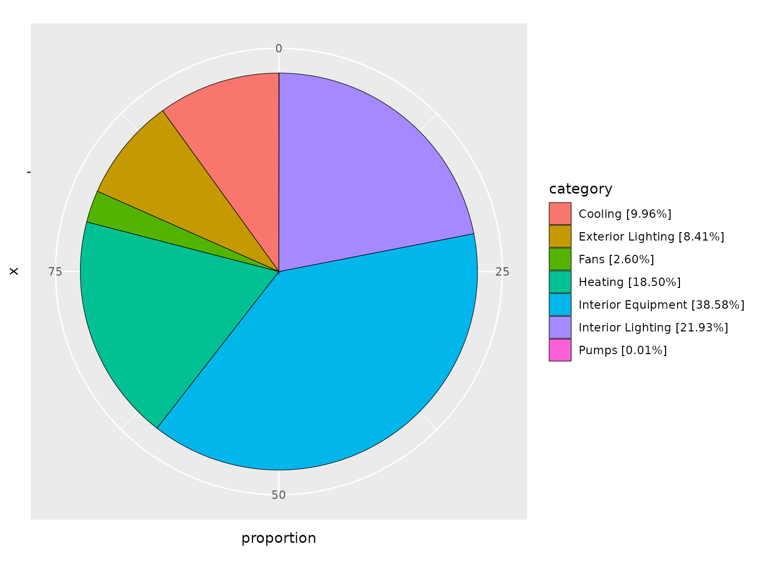
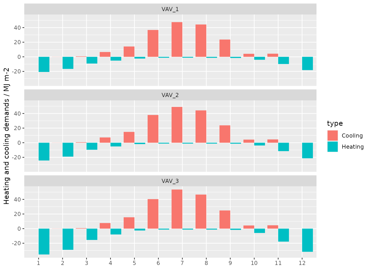
Get heating and cooling demand profile
# calculate air-conditioned floor area per storey
storey <- zones %>%
    # exclude plenum zones
    filter(is_part_of_total_area == 1) %>%
    # group by centroid height
    group_by(centroid_height = round(centroid_z, digits = 4)) %>%
    # calculate total floor area
    summarise(floor_area = sum(floor_area)) %>%
    ungroup() %>%
    # add storey index
    arrange(centroid_height) %>%
    mutate(storey = seq_len(n()), air_system = paste("VAV", storey, sep = "_")) %>%
    select(air_system, floor_area)

# get monthly heating and cooling demands per served area
aircon_out_mon <- aircon_out %>%
    # only consider weekdays
    filter(!day_type %in% c("Holiday", "Saturday", "Sunday")) %>%
    # add an identifier column to indicate cooling and heating condition
    mutate(type = case_when(
        grepl("Heating", name) ~ "Heating",
        grepl("Cooling", name) ~ "Cooling"
    )) %>%
    # add floor area served by each air-conditioning system
    left_join(storey, c("key_value" = "air_system")) %>%
    # calculate the monthly averaged heating and cooling demands in MJ/m2
    group_by(month, type, air_system = key_value) %>%
    summarise(system_output = sum(value) / 1e6 / floor_area[1]) %>%
    ungroup()
#> `summarise()` has regrouped the output.
#> ℹ Summaries were computed grouped by month, type, and air_system.
#> ℹ Output is grouped by month and type.
#> ℹ Use `summarise(.groups = "drop_last")` to silence this message.
#> ℹ Use `summarise(.by = c(month, type, air_system))` for per-operation grouping
#>   (`?dplyr::dplyr_by`) instead.

# plot a column chart to show the heating and cooling demand profile
aircon_out_mon %>%
    mutate(month = as.factor(month)) %>%
    mutate(system_output = case_when(
        type == "Heating" ~ -system_output,
        type == "Cooling" ~ system_output
    )) %>%
    ggplot() +
    geom_col(aes(month, system_output, group = type, fill = type), position = "dodge") +
    facet_wrap(vars(air_system), ncol = 1) +
    labs(x = "", y = "Heating and cooling demands / MJ m-2")